Visualisation
cf-plot
The cf-plot package provides
metadata-aware visualisation for cf fields. This is a seperate
library and cf does not depend on it.
The functionality of cfplot includes
- Cylindrical projection plots
- Polar stereographic plots
- Latitude/longitude - height plots
- Hovmuller plots
- Vector plots
- Stipple (significance) plots
- Multiple plots on a page
- Different colour scales
- User defined axes
- Rotated pole plots
- Irregular grid plots
- Graph plots
Examples
There are many and varied examples of using cf-plot with cf on the
cf-plot homepage (http://ajheaps.github.io/cf-plot/). Two simple
examples are shown here.
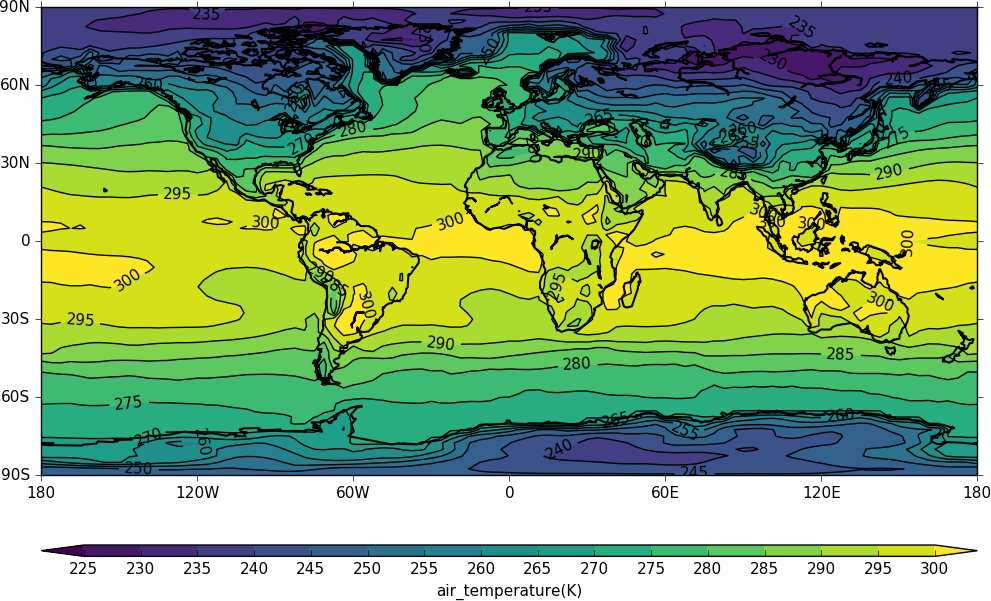
A simple 2-d contour plot could be produced as follows:
>>> import cf
>>> import cfplot
>>> f = cf.read_field('data1.nc')
>>> cfplot.con(f)
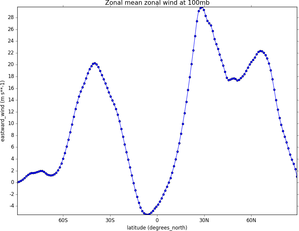
A simple 1-d line plot could be produced as follows:
>>> f = cf.read_field('data2.nc')
>>> cfplot.lineplot(f, marker='o', color='blue', title='Zonal mean zonal wind at 100mb')